Blinkit Data Analyst:
Blinkit hires data analysts on a large scale. Not only blinkit , if you are applying for the data science job roles at e-commerce. You must have a project on e-commerce.
This blog will focus from basic to advanced , how a data analyst find meaningful insights.
1. Understanding E-commerce Data
E-commerce data encompasses a wide array of information, including customer transactions, product details, user behavior, sales trends, and more. Before diving into analysis, it’s crucial to understand the structure and characteristics of e-commerce data. Common data sources in e-commerce include transaction logs, website analytics, customer reviews, and inventory databases.
2. Exploratory Data Analysis (EDA)
EDA serves as the foundation for uncovering insights from e-commerce data. Data Analyst employ various techniques such as summary statistics, data visualization, and correlation analysis to gain a deeper understanding of the data. EDA helps identify patterns, trends, outliers, and relationships within the dataset, laying the groundwork for further analysis.
3. Data Visualization and Reporting
Effective communication of insights is essential for driving actionable decisions within organizations. Data analysts leverage data visualization tools like Tableau, Power BI, or matplotlib to create visually compelling dashboards and reports. By presenting insights in a clear and intuitive manner, analysts empower stakeholders to make informed decisions and drive business success.
Load the Data
df = pd.read_csv('/kaggle/input/blinkit-grocery-list-price-city-date/blinkit_retail.csv')
df.head()
4. Get the info of the data
df.info()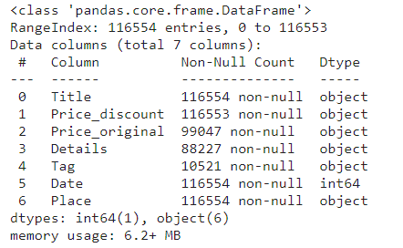
5. Converting Data To the right Data type
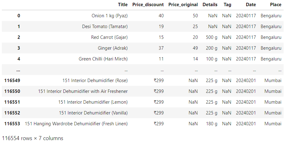
Data analyst would need to convert Price_discount and Price_original to float data type.
df['Price_discount'] = df['Price_discount'].str.replace('₹','').str.replace(',','')
df['Price_original'] = df['Price_original'].str.replace('₹','').str.replace(',','')
df
df['Price_discount'] = df['Price_discount'].astype(float)
df['Price_original'] = df['Price_original'].astype(float)
df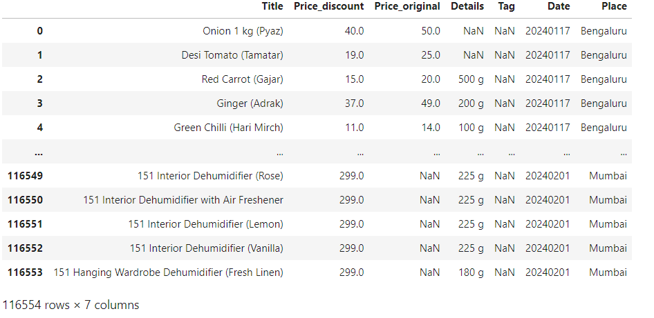
6. Converting Date Time
df['Date'] = pd.to_datetime(df['Date'],format='%Y%m%d')
df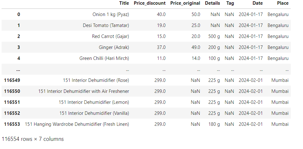
7. Price Analysis
- Data analyst Calculates the average, median, minimum, and maximum prices for both discounted and original prices.
avg_price_original = df['Price_original'].mean()
avg_price_discount = df['Price_discount'].mean()
med_price_original = df['Price_original'].median()
med_price_discount = df['Price_discount'].median()
min_price_original = df['Price_original'].min()
min_price_discount = df['Price_discount'].min()
max_price_original = df['Price_original'].max()
max_price_discount = df['Price_discount'].max()
print('Average Price Original',avg_price_original)
print('Average Price Discount',avg_price_discount)
print('Median Price Original',med_price_original)
print('Median Price Discount',med_price_discount)
print('Minimum Price Original',min_price_original)
print('Minimum Price Discount',min_price_discount)
print('Maximum Price Original',max_price_original)
print('Maximum Price Discount',max_price_discount)
Output :
- Average Price Original 646.6132038325239
- Average Price Discount 423.2343740615857
- Median Price Original 299.0
- Median Price Discount 200.0
- Minimum Price Original 14.0
- Minimum Price Discount 11.0
- Maximum Price Original 39900.0
- Maximum Price Discount 32899.0
- Identify products with the highest and lowest prices.
##Identify products with the highest and lowest prices.
expensive_prod_df = df.loc[df['Price_original']==df['Price_original'].max()]

lowest_prod_df = df.loc[df['Price_original']==df['Price_original'].min()]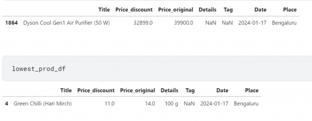
- Data analyst Determine the percentage discount offered on average.
df['Percentage'] = ((df['Price_original']-df['Price_discount'])*100)/50
ndf = df.groupby('Title').agg(
avg = ('Percentage','mean')
).reset_index().sort_values(by='avg',ascending=False)
ndf
8. Identify the top-selling products based on sales volume
- Data analyst identify the top-selling products, we can calculate the total sales volume for each product by summing up the quantities sold. The products with the highest total sales volume would be considered the top-selling products.
# Load the dataset
data = df

# Top-selling products based on sales volume
top_selling_products = data.groupby('Title')['Price_original'].count().sort_values(ascending=False).head(1)

# Categories or types of products that are more popular
# Assuming categories are not explicitly provided, we'll use the first word in the product title as the category
data['Category'] = data['Title'].str.split().str[0]
popular_categories = data.groupby('Category')['Price_original'].count().sort_values(ascending=False)

# Relationship between product details (weight) and prices
# Assuming product weight is in the 'Details' column
data['Weight'] = data['Details'].str.extract('(\d+\.?\d*) g')
data['Weight'] = pd.to_numeric(data['Weight'], errors='coerce')  # Convert to numeric
weight_price_relationship = data.groupby('Weight')['Price_original'].mean()

# Patterns or trends in product sales over time
data['Date'] = pd.to_datetime(data['Date'])
sales_over_time = data.groupby(['Date', 'Title'])['Price_original'].count().unstack().fillna(0)
sales_over_time.plot(legend=False, figsize=(10, 6), title='Product Sales Over Time')
9. Analyze which categories or types of products are more popular
- Data analyst can categorize products based on their type or category (e.g., fruits, vegetables, household items) and then calculate the total sales volume or revenue for each category. This will help us determine which categories are more popular among customers.
# Extract category from the product title
df['Category'] = df['Title'].str.split().str[0]

# Calculate total sales volume for each category
category_sales = df.groupby('Category')['Price_original'].count().sort_values(ascending=False)

print(category_sales)
10. Explore the relationship between product details (e.g., weight) and prices
- Data analyst can analyze how product details, such as weight, impact the prices of products. This can be done by visualizing the relationship between product weight and prices using scatter plots or by calculating correlation coefficients.
import pandas as pd
import matplotlib.pyplot as plt


# Extract relevant columns (product details and prices)
product_details = df['Details']  # Assuming 'Details' column contains product details (e.g., weight)
prices = df['Price_original']    # Assuming 'Price_original' column contains original prices

# Clean the data: handle missing values
df_cleaned = df.dropna(subset=['Details', 'Price_original'])

# Extract numeric values from product details (e.g., weight)
df_cleaned['Weight'] = df_cleaned['Details'].str.extract('(\d+\.?\d*) g')
df_cleaned['Weight'] = pd.to_numeric(df_cleaned['Weight'], errors='coerce')  # Convert to numeric

# Visualize the relationship between product weight and prices using scatter plot
plt.figure(figsize=(10, 6))
plt.scatter(df_cleaned['Weight'], df_cleaned['Price_original'], alpha=0.5)
plt.title('Relationship between Product Weight and Prices')
plt.xlabel('Product Weight (g)')
plt.ylabel('Price (Original)')
plt.grid(True)
plt.show()

# Calculate correlation coefficient (optional)
correlation_coefficient = df_cleaned['Weight'].corr(df_cleaned['Price_original'])
print("Correlation Coefficient:", correlation_coefficient)
11. Check for any patterns or trends in product sales over time
- Data analyst identify patterns or trends in product sales over time, we can plot the sales volume or revenue for each product over different time periods (e.g., daily, weekly, monthly). This will help us identify any seasonal variations, trends, or spikes in sales for specific products.
import pandas as pd
import matplotlib.pyplot as plt


# Convert the 'Date' column to datetime format
df['Date'] = pd.to_datetime(df['Date'])

# Group the data by date and product title to calculate total sales volume
sales_over_time = df.groupby(['Date', 'Title']).size().unstack(fill_value=0)

# Optionally, resample the data to aggregate sales over larger time periods (e.g., weekly or monthly)
# sales_over_time = sales_over_time.resample('W').sum()  # Weekly aggregation
# sales_over_time = sales_over_time.resample('M').sum()  # Monthly aggregation

# Plot the sales trends for each product
plt.figure(figsize=(12, 6))
for title in sales_over_time.columns:
    plt.plot(sales_over_time.index, sales_over_time[title], label=title)

plt.title('Product Sales Trends Over Time')
plt.xlabel('Date')
plt.ylabel('Sales Volume')
plt.legend(loc='upper left', fontsize='small', bbox_to_anchor=(1, 1))
plt.grid(True)
plt.show()
If you wish to learn more about data science or want to curve your career in the data science field feel free to join our free workshop on Masters in Data Science with PowerBI, where you will get to know how exactly the data science field works and why companies are ready to pay handsome salaries in this field.
In this workshop, you will get to know each tool and technology from scratch that will make you skillfully eligible for any data science profile.
To join this workshop, register yourself on consoleflare and we will call you back.
Thinking, Why Console Flare?
- Recently, ConsoleFlare has been recognized as one of the Top 10 Most Promising Data Science Training Institutes of 2023.
- Console Flare offers the opportunity to learn Data Science in Hindi, just like how you speak daily.
- Console Flare believes in the idea of “What to learn and what not to learn” and this can be seen in their curriculum structure. They have designed their program based on what you need to learn for data science and nothing else.
- Want more reasons


